Google Sheets, Google’s free spreadsheet tool, has been winning hearts across the globe, thanks to its seamless cloud integration, easy collaboration features, and rich set of functionalities. But as with most software, the more you dive deep, the more treasures you discover. One such gem is the “Dynamic Drop-Down List.” In this post, we’ll unravel the steps to create an auto-updating drop-down list and discuss why this feature can significantly level up your spreadsheet skills.
Why Dynamic Drop-Down Lists?
Imagine maintaining a roster of team members in a company. Employees come and go, and every time there’s a change, you have to manually update any drop-down lists referencing this roster. Time-consuming, right? What if the list updated itself automatically every time there’s a new entry or removal? That’s precisely the superpower Dynamic Drop-Down Lists bring to your Google Sheets!
Setting the Foundation: Named Ranges
Before we dive into creating our dynamic list, it’s essential to understand the concept of “Named Ranges” in Google Sheets. Named Ranges allow you to label a particular group of cells with a name, making it easier to reference in formulas.
- Creating a Named Range: Highlight the cells you want to name. Click on
Datain the top menu, selectNamed ranges..., and provide a name for your selected cells.
Crafting Your Dynamic Drop-Down List
With the foundation set, let’s craft our dynamic list:
- Start with Your Data: Before creating a drop-down, have a column where you’ll input your dynamic data. For our example, let’s consider a column where you list team members.
- Expand the Named Range: Instead of defining a named range for only the existing names, anticipate future entries. If you have ten team members now but expect it to go up to 50, define the range to encompass 50 cells.
- Create a Dynamic Formula:
- In a new column or cell, use the formula
=UNIQUE(FILTER(A:A, A:A<>""))(assuming your data starts in column A). This formula removes duplicates and blanks, ensuring your drop-down list remains clean.
- Crafting the Drop-Down:
- Select the cell or range of cells where you want the drop-down list.
- Click on
Dataand thenData validation. - Under criteria, choose ‘List from a range’ and then enter the range of your dynamic formula.
- Test Your Dynamic Drop-Down: As you add or remove team members from your original list, you’ll notice the drop-down list automatically updating itself!
Benefits of Dynamic Drop-Downs
- Time-Saving: Once set, these lists require minimal maintenance, saving you time in the long run.
- Error Reduction: By automating updates, you reduce the risk of manual errors creeping into your sheets.
- Enhanced Presentation: Dynamic lists, being cleaner with no duplicates or blanks, make your spreadsheet look more professional.
- Scalability: As your data grows, your drop-downs automatically adapt without needing constant tweaking.
Limitations and Workarounds
While dynamic drop-down lists are mighty, they aren’t without their constraints. One notable limitation is that if you delete a name from the middle of your list, it might create a blank space. However, using the UNIQUE and FILTER combo, as shown above, usually takes care of such issues.
Conclusion
Google Sheets continues to prove its mettle as more than just a basic spreadsheet tool. The capability to create dynamic drop-down lists is a testament to its evolving features tailored to enhance user efficiency. Whether you’re an occasional user or someone knee-deep in data analysis, understanding and leveraging these dynamic lists can significantly boost your Google Sheets prowess. So, the next time you’re working on a project, remember this nifty trick and let your lists evolve as dynamically as your data does!


I can’t seem to make this work. Everytime I specify the dynamic range to be used, Sheets hard codes the name references in its drop down.
I have three values in Cells A4, A5 and A6… that are dynamically updated based on values that are looked up based on what is in cell A1..
the data validation to create a drop down points to the range of A4, A5 and A6 but it takes whatever values that are listed at the time and creates the drop down list based on them.
If the values change again the drop down list breaks.